
One of the reasons to use any kind of project management methodology is to reduce costs.
A delay in a single week of a project creates two different cost types:
- The first is the cost of the team, since they will need to work another week.
- The second is the Cost of Delay, which is the income not collected due to the delay. For instance, suppose the new feature this team is working on would generate a daily income of $100, the Cost of Delay would be $700 ($100 * 7 days).
Since these costs can be high, using tools that provide more visibility on delivery dates is necessary. One tool that can help solve this problem is the Gantt Chart. With the Gantt Chart it’s possible to identify the most frail points of the project (the critical path) where more effort should be made to prevent delays, since a delay in any step of those points will impact the project as a whole.
Even though this tool is great for some types of projects (normally when there is a low uncertainty level), it’s not ideal for projects where the predictability is low due to the variance of the deliverables, as in projects that happen in the field of knowledge (writing a book or software development, for example).
Here at Plataformatec, we have always done our best to make our delivery predictions based on data and ensure they follow proven scientific methodology. The two methods we use the most are:
- Linear Progression
- Monte Carlo Simulation
LINEAR PROGRESSION
In linear progression, we do data analysis on the delivered work items during some time period (in software development we normally work with weeks) and through the study of this information we come up with the best values for the progression. For example: suppose we have the following historic values of work items by week, as shown below:
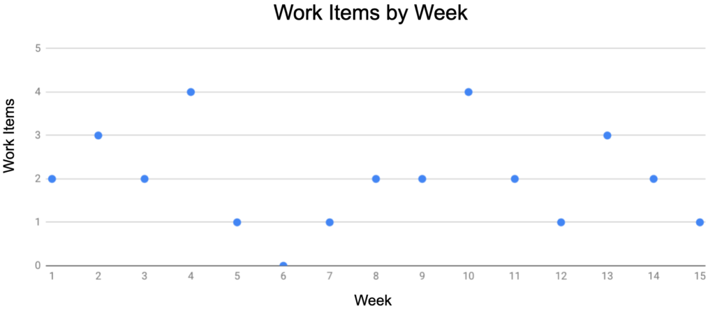
A value that could be used as a pessimistic projection would be to assume a delivery of 1 work item per week, seeing as we’ve had 5 cases where the throughput was 1 or 0. For the optimist projection we could use either the value of 3 or 4, or even 3.5, as we’ve had 4 instances where the throughput was 3 or higher. Lastly, for the likely projection, a good value would be 2, as it’s the median and the mode of this dataset.
The biggest problem with the linear progression is that we are inputting the values for each scenario, something that can be dangerous if the person operating the linear progression doesn’t have a good grasp of data analytics. Furthermore, linear progression ignores variance. Thus, in work systems with high variance of deliveries, the linear progression tool might not be the best approach.
MONTE CARLO
Another technique we can use is called Monte Carlo, which runs random picks from our historic throughput data to try and find the likelihood of delivery.
I’m having success using this method, however a question that keeps coming to my mind is: “How many interactions are necessary to make the method statistically valuable and the results reliable?”. Looking for an answer to this question, I’ve researched some statistics books, and also the internet, but wasn’t able to find any information that would help.
So I decided to run a study on this subject. Monte Carlo’s objective is to infer the probability of an event, “forcing” it to happen so many times, in order to use the law of large numbers in our favor. For example, if you flip a coin a thousand times, count how many times it falls as “heads”, and divide by a thousand, you will get an inference of the probability of getting “heads”.
To check the quality of the method, I first ran tests over probabilities for which I already knew the expected results. After that, I started increasing the complexity of the problem, in order to see if there was any correlation between the difficulty of a problem and the number of interactions necessary for the inferred value from Monte Carlo to be as close as possible to the calculated one.
The objective of the tests is to see how many interactions are necessary for the inferred value to be close enough to the calculated value that the gain of running more interactions would be too low to compensate the computer power necessary to run it (for a project probability standpoint an error in the first or second decimal values would be acceptable). I’d like to highlight that this blog post is not a scientific study of the subject, and the objective is to understand through inference a good value for project predictions.
THE TESTS
The tests were performed using the programing language R, which can be downloaded in this link. If you would rather use an IDE, I recommend using RStudio.
In each test, I’ve run the algorithm 100 times using the following interaction values: 100 (one hundred), 1000 (one thousand), 10000 (ten thousand), 100000 (one hundred thousand), 1000000 (one million), 10000000 (ten million), 100000000 (one hundred million) e 200000000 (two hundred million). The results of these 100 “rounds” are then consolidated.
THE COIN
The first test that I’ve run was the flipping of a single coin. In a coin flip, there is a 50% chance of it landing on any side, and this is the value we want the Monte Carlo to infer. For that I’ve used the following R code:
FLipCoin <- function(iterations)
{
# Creates a vector with the possible values for a coin 1 = Heads and 0 = Tails
coin = c(0,1)
result = 0
# Flips a number of coins equal to the interaction value and sum up all the times where the coin landed in "Heads"
result = sum(sample(coin, iterations, replace=T))
# Turns the value in a percentage of the coin flips
result = (result/iterations) * 100
return(result)
}
# Initiates variables
result_vector = 0
time_vector = 0
control = 0
# Controls the interaction quantity
iterations = 100
# Alocates the percentual of "Heads" results in a 100 size vector and the execution time in another
while(control != 100)
{
start_time = Sys.time()
result_vector = append(result_vector, FLipCoin(iterations))
finish_time = Sys.time()
time = finish_time - start_time
time_vector = append(time_vector, time)
control = control + 1
}
# Shows the percentual of "Heads"
result_vector
# Shows the execution times
time_vector
Code language: PHP (php)Changing the values of the iterations and compiling the results, I’ve got the following table:
-
Iterations Min result Max result Expected result Average result Average result - Expected result Result's median Result's median - Expected result | Result's Standard deviation 100 33.00000 67.00000 50.00000 50.02000 0.02000 50.00000 0.00000 5.09368 1000 43.60000 56.20000 50.00000 49.99440 0.00560 50.00000 0.00000 1.59105 10000 48.35000 51.78000 50.00000 50.01263 0.01263 50.02000 0.02000 0.51001 100000 49.58000 51.78000 50.00000 49.99110 0.00890 49.99350 0.00650 0.15805 1000000 49.85170 50.15090 50.00000 49.99883 0.00117 49.99785 0.00215 0.04811 10000000 49.95433 50.05807 50.00000 50.00013 0.00013 50.00010 0.00010 0.01564 100000000 49.98435 50.01637 50.00000 50.00004 0.00004 49.99989 0.00011 0.00516 200000000 49.98890 50.01195 50.00000 49.99981 0.00019 49.99987 0.00013 0.00345
In the instance of a simple problem, like the flipping of a single coin, we can see that a good iteration value could be:
- between 10M and 100M if you are ok with having an error in the third decimal,
- between 100k and 1M in the second decimal
- between 1k and 10k in the first decimal.
ONE DICE
With the coin test it was possible to infer the number of necessary interactions, based on the desired degree of reliability. However a question remains regarding if this behavior changes for more complex problems. Because of that, I’ve run a similar test with a single six-sided die that has a 16,67% chance of landing on any side.
RollDie <- function(iterations)
{
# Creates a vector with the possible values of the die
die = 1:6
result = 0
# Alocates the die roll results
result = sample(die,iterations,replace=T)
# Sum up every instace where the die landed on 6
result = sum(result == 6)
# Turns the value in a percentage of the die rolls
result = (result/iterations) * 100
return(result)
}
# Initiates variables
result_vector = 0
time_vector = 0
control = 0
# Controls the interaction quantity
iterations = 100
# Alocates the percentual of "6" results in a 100 size vector and the execution time in another
while(control != 100)
{
start_time = Sys.time()
result_vector = append(result_vector, RollDie(iterations))
finish_time = Sys.time()
time = finish_time - start_time
time_vector = append(time_vector, time)
control = control + 1
}
# Shows the percentual of "6"
result_vector
# Shows the execution times
time_vector
Code language: PHP (php)Changing the values of the iterations and compiling the results , I’ve got the following table:
| Iterations | Min result | Max result | Expected result | Average result | Average result - Expected result | Result's median | Result's median - Expected | result | Result's Standard deviation |
|---|---|---|---|---|---|---|---|---|
| 100 | 33.00000 | 67.00000 | 50.00000 | 50.02000 | 0.02000 | 50.00000 | 0.00000 | 5.09368 |
| 1000 | 43.60000 | 56.20000 | 50.00000 | 49.99440 | 0.00560 | 50.00000 | 0.00000 | 1.59105 |
| 10000 | 48.35000 | 51.78000 | 50.00000 | 50.01263 | 0.01263 | 50.02000 | 0.02000 | 0.51001 |
| 100000 | 49.58000 | 51.78000 | 50.00000 | 49.99110 | 0.00890 | 49.99350 | 0.00650 | 0.15805 |
| 1000000 | 49.85170 | 50.15090 | 50.00000 | 49.99883 | 0.00117 | 49.99785 | 0.00215 | 0.04811 |
| 10000000 | 49.95433 | 50.05807 | 50.00000 | 50.00013 | 0.00013 | 50.00010 | 0.00010 | 0.01564 |
| 100000000 | 49.98435 | 50.01637 | 50.00000 | 50.00004 | 0.00004 | 49.99989 | 0.00011 | 0.00516 |
| 200000000 | 49.98890 | 50.01195 | 50.00000 | 49.99981 | 0.00019 | 49.99987 | 0.00013 | 0.00345 |
We can see that in this case, the iteration values are the same as for the instance of the coin toss, where a good value could be something between 10M and 100M if you need to have an error in the third decimal, between 100k and 1M for an error in the second decimal and between 1k and 10k for an error in the first decimal.
This test result shows that, either the complexity of the problem has no influence on the number of interactions or that both problems (coin toss and single die roll) have similar complexity levels.
Analyzing the execution times for both problems, it’s possible to see that they took about the same time. This also corroborates with the hypothesis that they have similar complexity levels.
TWO DICE
To test the hypothesis that the complexity of the above problems were too close, and this was the reason for the interaction values to be close, I’ve decided to double the complexity of the die roll problem by rolling two dice instead of only one (it’s important to note that doubling the quantity of functions doesn’t always mean that the complexity order will double as well, as it depends on the Big-O Notation). The highest probability value for two dice is 7, with a 16,67% chance of occurrence.
RollsTwoDice <- function(iterations)
{
  # Creates a vector with the possible values of the die
  die = 1:6
  result = 0

  # Alocates the die roll results
  first_roll = sample(die,iterations,replace=T)
  second_roll = sample(die,iterations,replace=T)

  # Sum the vector values position-wise
  result = first_roll + second_roll

  # Sum up every instace where the dice landed on 7
  result = sum(result == 7)

  # Turns the value in a percentage of the dice rolls
  result = (result/iterations) * 100

  return(result)
}

# Initiates variables
result_vector = 0
time_vector = 0
control = 0

# Controls the interaction quantity
iterations = 100

# Alocates the percentual of "7" results in a 100 size vector and the execution time in another
while(control != 100)
{
  start_time = Sys.time()
  result_vector = append(result_vector, RollsTwoDice(iterations))
  finish_time = Sys.time()

  time = finish_time - start_time
  time_vector = append(time_vector, time)

  control = control + 1
}

# Shows the percentual of "7"
result_vector

# Shows the execution times
time_vector
Code language: PHP (php)
Changing the values of the iterations and compiling the results, I’ve got the following table:
| Iterations | Min result | Max result | Expected result | Average result | Average result - Expected result | Result's median | Result's median - Expected | result | Result's Standard deviation |
|---|---|---|---|---|---|---|---|---|
| 100 | 6.00000 | 28.00000 | 16.66667 | 16.58100 | -0.08567 | 16.00000 | -0.66667 | 3.64372 |
| 1000 | 13.20000 | 20.40000 | 16.66667 | 16.68500 | 0.01833 | 16.60000 | -0.06667 | 1.16949 |
| 10000 | 15.60000 | 17.94000 | 16.66667 | 16.65962 | -0.00705 | 16.67000 | 0.00333 | 0.38072 |
| 100000 | 16.22200 | 17.06200 | 16.66667 | 16.66109 | -0.00557 | 16.66500 | -0.00167 | 0.11356 |
| 1000000 | 16.54960 | 16.54960 | 16.66667 | 16.66616 | -0.00050 | 16.66790 | 0.00123 | 0.03650 |
| 10000000 | 16.63294 | 16.70266 | 16.66667 | 16.66607 | -0.00060 | 16.66577 | -0.00090 | 0.01220 |
| 100000000 | 16.65592 | 16.67948 | 16.66667 | 16.66670 | 0.00004 | 16.66679 | 0.00012 | 0.00372 |
| 200000000 | 16.65787 | 16.67476 | 16.66667 | 16.66671 | 0.00004 | 16.66671 | 0.00004 | 0.00267 |
Again we find the same interaction quantity for each error level. In the case of this problem it’s possible to identify that it was more complex since the execution for 200M took on average 7.47 seconds longer when compared to the single die roll.
FIVE DICE
The inference that I’ve built until this point is that the complexity of the problem influences very little in the iteration quantities, but to be sure of that, I ran one last test with 5 dice. The highest probability when rolling five dice is the values of 17 and 18, with 10.03% probability each.
Since this problem is a lot more complex than the others I’ve decided to run only 10 times each instead of 100.
RollsFiveDice <- function(iterations)
{
  # Creates a vector with the possible values of the die
  dado = 1:6
  result = 0

  # Alocates the die roll results
  first_roll = sample(dado,iterations,replace=T)
  second_roll = sample(dado,iterations,replace=T)
  terceira_rolagem = sample(dado,iterations,replace=T)
  quarta_rolagem = sample(dado,iterations,replace=T)
  quinta_rolagem = sample(dado,iterations,replace=T)

  # Sum the vector values position-wise
  result = first_roll + second_roll + terceira_rolagem + quarta_rolagem + quinta_rolagem

  # Sum up every instace where the dice landed on 18
  result = sum(result == 18)

  # Turns the value in a percentage of the dice rolls
  result = (result/iterations) * 100

  return(result)
}

# Initiates variables
result_vector = 0
time_vector = 0
control = 0

# Controls the interaction quantity
iterations = 10

# Alocates the percentual of "18" results in a 100 size vector and the execution time in another
while(control != 100)
{
  start_time = Sys.time()
  result_vector = append(result_vector, RollsFiveDice(iterations))
  finish_time = Sys.time()

  time = finish_time - start_time
  time_vector = append(time_vector, time)

  control = control + 1
}

# Shows the percentual of "18"
result_vector

# Shows the execution times
time_vector
Code language: PHP (php)
Changing the values of the iterations and compiling the results, I’ve got the following table:
| Iterations | Min result | Max result | Expected result | Average result | Average result - Expected result | Result's median | Result's median - Expected result | Result's Standard deviation |
|---|---|---|---|---|---|---|---|---|
| 100 | 5.00000 | 31.00000 | 16.66667 | 16.37100 | -0.29567 | 16.00000 | -0.66667 | 3.77487 |
| 1000 | 13.40000 | 21.80000 | 16.66667 | 16.64710 | -0.01957 | 16.60000 | -0.06667 | 1.18550 |
| 10000 | 15.33000 | 17.77000 | 16.66667 | 16.68307 | 0.01640 | 16.68500 | 0.01833 | 0.38059 |
| 100000 | 16.23100 | 17.06600 | 16.66667 | 16.66546 | -0.00120 | 16.66800 | 0.00133 | 0.11597 |
| 1000000 | 16.54450 | 16.81170 | 16.66667 | 16.66657 | -0.00010 | 16.66860 | 0.00193 | 0.03798 |
| 10000000 | 16.62888 | 16.70282 | 16.66667 | 16.66683 | 0.00016 | 16.66705 | 0.00038 | 0.01155 |
| 100000000 | 16.65408 | 16.67899 | 16.66667 | 16.66669 | 0.00002 | 16.66673 | 0.00007 | 0.00382 |
| 200000000 | 16.65881 | 16.67455 | 16.66667 | 16.66675 | 0.00009 | 16.66682 | 0.00015 | 0.00258 |
Once again we can see that the values for the iterations are the same as above. It’s possible to notice that this problem is clearly more complex, as it took 35 seconds longer when compared to the roll of a single die.
CONCLUSION
After running those tests, it’s possible to conclude that for the use on project management, a good iteration value would be somewhere between 1k and 100M, depending on the error level as shown below:
- Error in the first decimal: 1k to 10k
- Error in the second decimal: 100k to 1M
- Error in the third decimal: 10M to 100M
The value that I’ve been using is 3M, for stakeholder reports. However, when I’m running the method for my own analysis, I use a lower value, somewhere between 250k and 750k.
How about you? Have you tried to run Monte Carlo Simulations? How many iterations are you using? Tell us in the comment section below or on Twitter @plataformatec.