Nowadays we are using a more probabilistic approach to manage our processes than deterministic. That means that we use different statistical methods to predict the future instead of blind estimations. But wait… wasn’t unpredictability one of the main reasons that made us change from Waterfall to Agile?
Yes, uncertainty is inherent to software development. For example, one could not possibly predict all the features of a system at the beginning of a project.
But what if we could forecast how just the next few weeks would behave?
That is what we are trying to achieve using a gathering of metrics and running Monte Carlo simulation over them.
To understand how we collect our metrics, I recommend you read these posts:
- Why we love metrics? Learning with lead time
- Why we love metrics? Throughput and burnup charts
- Why we love metrics? Cumulative flow diagrams
Most people don’t use any metrics to manage their projects. You can then imagine how many use complex statistical models to forecast a project completion. However, having this knowledge on your current project will help you deliver faster and better.
In this post, you will see how we went from a naive forecast approach to a more precise and robust one using Monte Carlo Simulation. Moreover, we’ll explain how Monte Carlo simulation works in an easy and straightforward way and then make an analogy between the simple example and our real world approach. Knowing when your project will likely end can help you manage the project’s budget, give better feedbacks to stakeholders and give you the confidence that you are indeed in control of your project.
Why not other methods?
We have been playing with other methods of forecasting for a long time, and all of them had some drawbacks. Here we list some of them and how and why we opted to use Monte Carlo.
Mean Throughput
Some of you might have thought of a simple method in which we would use the average throughput to forecast the end of the project. However, as you can see on this blog post Power of the metrics: Don’t use average to forecast deadlines, that would be an extremely naive method, and it doesn’t work.
Linear Regression Approach
As a first approach, we used linear regression, based on our accumulated throughput, to forecast when a project would end:
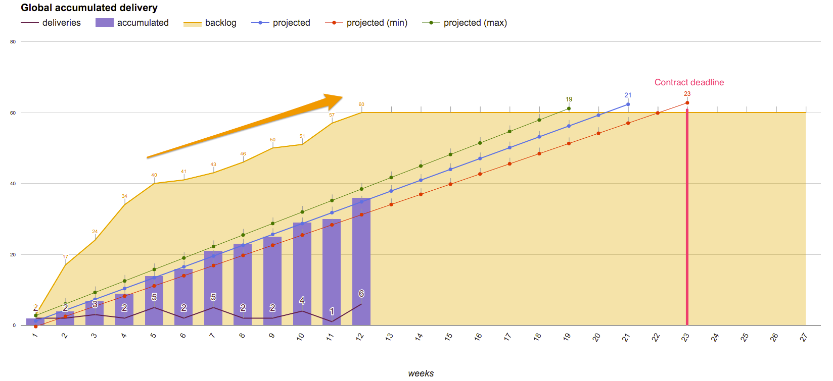
However, we identified two different problems that we were not considering when doing that analysis:
- We had to maintain the number of items in our backlog constant for the forecasting to work, which is very biasing.
- We discovered, after some analysis, that both throughput and lead times do not follow a normal distribution, thus it would not make sense to calculate a linear regression (See on Looking at Lead Time in a different way and Assumptions of Linear Regression).
Manual Setting Approach
Firstly, we focused on avoiding problem number 2, and we started using a more parsimonious model, which used methods that we knew were somehow skewed, but we could better control them.
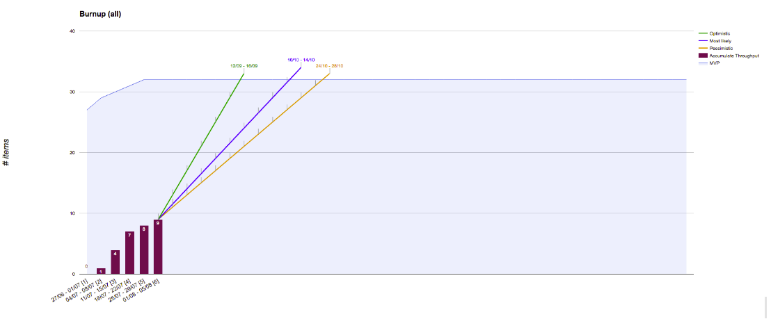
We manually added the throughput performance that would cause each different forecast to reach the backlog in a certain date. This forecasting approach comes from the study of percentiles of our throughput history.
We had better results with that, since we could change the forecast manually and, therefore, tune it according to the current state of the project. But the problem number 1, the fact that we were not considering the change in the backlog, made us take a step further and try Monte Carlo Simulation.
Monte Carlo Simulation
Wikipedia defines Monte Carlo method as
Monte Carlo methods vary, but tend to follow a particular pattern:
- Define a domain of possible inputs.
- Generate inputs randomly from a probability distribution over the domain.
- Perform a deterministic computation on the inputs.
- Aggregate the results.
It may seem difficult or complex at first but it is actually much simpler than it looks. You can look at it as the brute force method of forecasting. We’ll present a simple example and then show how we did in the real world. There’s a very good simulation made by Larry Maccherone that can elucidate it even more.
Dice Game
Imagine you are playing a dice game in which the goal is to reach a sum of 12 points with the least number of rolls. The best play here would be 2 consecutive rolls in which you get a 6 in both of them, and the worst would be 12 rolls getting a 1. What we want to calculate is the probability of ending the game after N runs.
Considering that we have 6 possible outcomes for each dice roll, the 6 faces of the dice, what is the probability of finishing the game in 1 roll?
Zero. Since you cannot get to 12 points if the dice goes only up to 6 points.
What about in the second roll?
It is the probability of getting two consecutive 6, which is basic statistics:
What about in the third roll?
You can achieve 12 points in many ways now, some of them are: (3,3,6), (3,4,5), (3,5,4), (3,4,6), (5,5,2), (4,4,4) and etc. Now the statistics behind that calculation are not that straightforward, right? That is when Monte Carlo simulation comes handy.
What Monte Carlo does is to simulate thousands dice rolls and then analyze the outcome. For example, to know the probability of finishing the game on the third round, it would roll the dice three times, sum the points and store that result. After that, it would repeat those steps 5000 times and summarize how many rolls each sum of points got:
| Sum of 3 dice rolls | How many times it appeared |
|---|---|
| 3 | 21 |
| 4 | 70 |
| 5 | 134 |
| 6 | 240 |
| 7 | 370 |
| 8 | 509 |
| 9 | 581 |
| 10 | 586 |
| 11 | 636 |
| 12 | 538 |
| 13 | 476 |
| 14 | 375 |
| 15 | 226 |
| 16 | 139 |
| 17 | 74 |
| 18 | 25 |
Now what it does is to sum all the occurrences that generated a sum greater than 12 and divide it by the total number of occurrences. In this case:
The same way we did it for the third round, we could do it for the fourth, fifth, and so on.
Real World
The real world solution is very similar to the dice rolling example. The only difference is that we vary the goal as well (the 12 points in the game scenario), to consider the change in the backlog.
So now the possible outcomes for each round (the sides of our dice) are our throughput history. And in the same way, we are “rolling dices” for our throughput, we need to roll the dices for our backlog in order to give it the chance to grow as well. In this case, the possible outcomes would be the Backlog Growth Rates (BGR).
Let’s start slowly. Let’s say our project history was this:
| Week Number | Throughput History | Backlog History |
|---|---|---|
| 1 | 2 stories | 15 stories (BGR: 0) |
| 2 | 3 stories | 17 stories (BGR: 2) |
| 3 | 0 stories | 18 stories (BGR: 1) |
| 4 | 2 stories | 19 stories (BGR: 1) |
| 5 | 5 stories | 21 stories (BGR: 2) |
| 6 | 0 stories | 22 stories (BGR: 1) |
| 7 | 1 stories | 22 stories (BGR: 0) |
| 8 | 3 stories | 24 stories (BGR: 2) |
| 9 | 3 stories | 24 stories (BGR: 0) |
So our possible plays each round for the throughput would be the set {2,3,0,2,5,0,1,3,3} and for the backlog would be {0,2,1,1,2,1,0,2,0}. We do not exclude repeated numbers because, with them, we can maintain the higher probability of having a number instead of others.
Now, we can apply the same rationale behind the dice game here. What is the probability of the total throughput reaching the same amount as the backlog, or more, in the first week? Some of the possible outcomes are the following:
| Throughput “Roll” | BGR “Roll” | Throughput Sum | Backlog Sum |
|---|---|---|---|
| 2 | 0 | 19+2 = 21 | 24 + 0 = 24 |
| 2 | 2 | 19+2 = 21 | 24 + 2 = 26 |
| 2 | 1 | 19+2 = 21 | 24 + 1 = 25 |
| 3 | 0 | 19+3 = 22 | 24 + 0 = 24 |
| 3 | 2 | 19+3 = 22 | 24 + 2 = 26 |
| 3 | 1 | 19+3 = 22 | 24 + 1 = 25 |
| 0 | 0 | 19+0 = 19 | 24 + 0 = 24 |
| 0 | 2 | 19+0 = 19 | 24 + 2 = 26 |
Then we would run many like those and see how many of them have a throughput sum greater than the backlog sum, and then divide the result by the number of runs. Doing that we would have the probability of the project ending in the first week. For the next week we would do the same but then rolling the dice twice in each round and summing them for both the throughput and the backlog.
One problem that this method had, was that the backlog at the beginning of a project behaves differently than at the middle or end of it. At the beginning, usually the growth is much faster because we are better understanding the problems and nuances of our project, at the end, the growth is basically from refining stories.
To solve this problem, instead of considering the whole BGR history as the possible outcome, we consider only the last 10 BGRs from the backlog, which would give us a better perspective on how the backlog is behaving lately.
The result for the next 10 weeks, using the new last-ten-BGR approach, is represented in the chart:
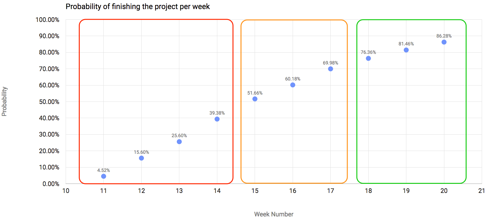
As you can see, I highlighted three different areas of the chart to illustrate what I think could be a takeaway from the chart:
- The first area, the red one, are the weeks in which we have less than 50% probability of finishing the project. Which means that it would be too risky to tell the stakeholders of your project that you would finish it in the next 4 weeks.
- The next area, the orange one, illustrates the weeks in which we have a probability between 50% and 75% of finishing the project. I would say that, if the stakeholders are pressuring you to deliver fast, those are the weeks that, if you take a leap of faith, you could finish.
- The green area is a more risk-free one, where you have a probability greater than 75% of completing the project. I would suggest that you always give preference to estimate the end of your project based on this area than the other ones, but we all know that we cannot always be that safe.
We tested the Monte Carlo simulation in past projects and it seems to work really well, but, as in any other statistical method, it gets much better after some weeks in the project than at the beginning.
Summary
Forecasting when a project is likely to end seems too “hokus-pokus”, but this method is really easy to implement and gives us a much better forecast and understanding of our project. It is important to make it clear that this method is a statistical method, thus it is not fail proof. The main goal is to add one more element into our toolkit and make project management a little bit easier.
In order to help you forecast software projects’ completion date, we are making a simple version of our spreadsheet available for you to download, so you can run simulations without much work.
To learn more about Monte Carlo Simulation, I recommend these great references:
- Troy Magennis’ book – Forecasting and Simulating Software Development Projects: Effective Modeling of Kanban & Scrum Projects using Monte-carlo Simulation
-
Daniel Vacanti’s website, book and blog: Actionable Agile
How are you forecasting the end of your project? What is your opinion about our approach? Share your thoughts with us in the comments below!